Biobank Intro Series: All of Us Observational Data (Part II)

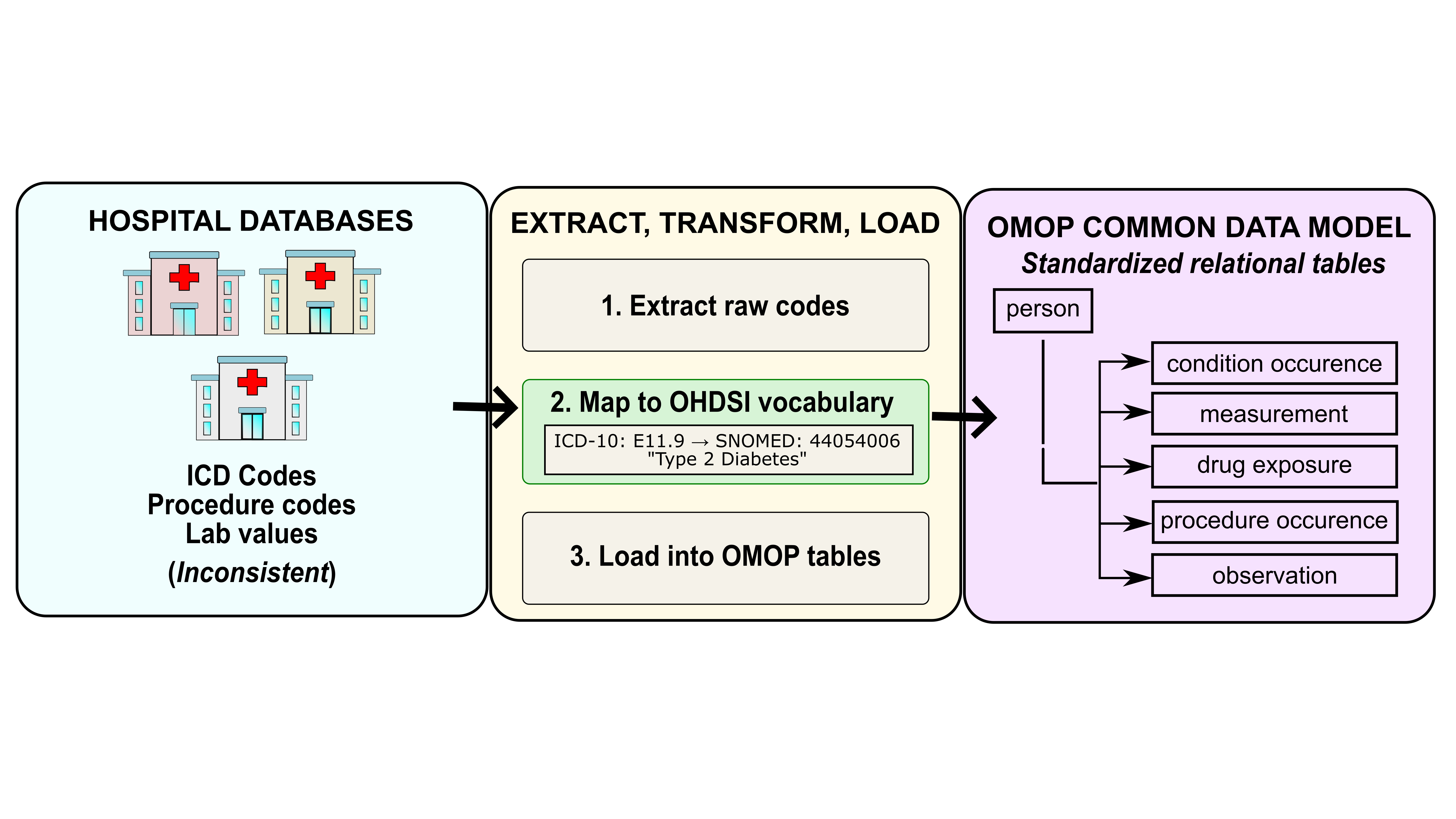
The UK has a single national health system, and it shows: one table, one field ID, a coding dictionary if you needed it. The US has hundreds of hospital systems, dozens of billing standards, and its data model matches this beloved chaotic energy. In All of Us, your data is spread across clinical tables, the coded values in those tables are translated via a separate concept table, and everything traces back to person_id. More joins, more steps, but it’s just what a data model built on real EHR data looks like.

With your concept IDs in hand (Part I), the workflow has three moving parts: knowing which clinical table holds your concept, joining to the concept table to decode any coded values, and merging everything back to person to build your cohort. More pieces than UKB, but engineered for the diverse US healthcare system.

The OMOP-CDM Schema

The full OMOP CDM schema is worth bookmarking. It documents every available table and its fields. Clinical tables contain records of observed medical and clinical data, where each row represents a single clinical event. In my experience, most analyses only touch a handful of clinical tables:

• condition_occurrence: diagnoses observed by a provider or reported by a patient
• measurement: lab values and test results (e.g., BMI, blood pressure)
• observation: clinical facts that cannot be measured with a standardized test, such as medical history, family history, and lifestyle choices
• drug_exposure: medication records, useful for validating diagnoses or identifying undiagnosed conditions

The person table is the anchor table of the schema. It holds one row per participant, and every clinical table links back to it via person_id. Like clinical tables, it also uses concept_id columns as foreign keys to the concept table for decoding coded values.

Query a Clinical Table

The OMOP CDM tables live in Google BigQuery. The examples below use Python’s pandas.read_gbq function, which takes a SQL string and returns a dataframe. R users can likely query them with the bigrquery package. The examples assume the following setup:

import pandas as pd
import os
CDR = os.environ['WORKSPACE_CDR']

In Part I, we found that systolic blood pressure maps to concept ID 3004249 in the measurement table. Let’s use that as our worked example:

sbp_query = f'''
    SELECT
        measurement_id,
        person_id,
        measurement_concept_id,
        measurement_type_concept_id,
        measurement_date,
        measurement_datetime,
        value_as_number
    FROM `{CDR}.measurement`
    WHERE measurement_concept_id = 3004249'''
sbp_df = pd.io.gbq.read_gbq(sbp_query, dialect='standard')
sbp_df

The SELECT statement exports these columns:

• measurement_id: unique row identifier
• person_id: foreign key linking the person and clinical tables
• measurement_concept_id: ID of the data field
• measurement_type_concept_id: ID of the data source (eg. EHR, Lab result, etc.)
• measurement_date / measurement_datetime: date and time of the record
• value_as_number: numeric systolic blood pressure value

The WHERE clause limits the measurement table to this field. Since we will stack multiple measurement types into a single cohort table, human-readable labels for measurement_concept_id and measurement_type_concept_id are essential for distinguishing which rows belong to which measurement.

Decode Coded Values via the concept Table

Coded fields across all OMOP tables store numeric IDs. To translate them, join to the concept table. The query below decodes the systolic blood pressure measurements:

sbp_query = f'''SELECT
  m.person_id,
  mc.concept_name AS measurement_name,
  mtc.concept_name AS measurement_type_name,
  m.value_as_number,
ROW_NUMBER() OVER (
    PARTITION BY m.person_id, m.measurement_concept_id
    ORDER BY m.measurement_date DESC, m.measurement_datetime DESC, m.measurement_id DESC
  ) AS recency_rank
FROM
  `{CDR}.measurement` m
LEFT JOIN `{CDR}.concept` mc ON mc.concept_id = m.measurement_concept_id
LEFT JOIN `{CDR}.concept` mtc ON mtc.concept_id = m.measurement_type_concept_id
WHERE measurement_concept_id = 3004249'''
pd.io.gbq.read_gbq(sbp_query, dialect='standard')

This JOIN pattern repeats throughout OMOP and works the same way for any coded field across any clinical table, including the person table. The query below decodes gender values:

gender_query = f'''
  SELECT
    person.person_id,
    pgc.concept_name as gender,
    person.gender_source_value,
    pgsc.concept_name as gender_source_concept_name
  FROM `{CDR}.person` person
  LEFT JOIN `{CDR}.concept` pgc ON pgc.concept_id = person.gender_concept_id
  LEFT JOIN `{CDR}.concept` pgsc ON pgsc.concept_id = person.gender_source_concept_id
'''
gender_df = pd.io.gbq.read_gbq(gender_query, dialect='standard')
gender_df

The gender_source_value column is the shortcut that feels right but isn’t. It contains raw, unstandardized values from the original data source, think of it as the “close enough” column. For any real analysis, always use the decoded gender column obtained through the concept join. Keep gender_source_value around for reference, but DO NOT let it anywhere near your results.

Merge Everything into a Cohort Table

Each query produces its own dataframe. Merge them on person_id to build your cohort:

cohort_df = pd.merge(
  gender_df,
  sbp_df.sort_values('recency_rank').drop_duplicates('person_id'),
  on='person_id',
  how='left'
)

This pattern scales to any study: find your concept IDs (Part I), query the relevant OMOP tables, join to concept for readable labels, and merge the resulting dataframes in pandas.

The pandas approach above is readable and easy to follow, but it loads each table into memory separately before joining. For larger cohorts, it’s more efficient to do the join entirely in SQL so BigQuery returns only the final result:

cohort_query = f'''
-- Pull one row per participant from the person table
SELECT
  p.person_id,
  pgc.concept_name AS gender,
  p.gender_source_value AS raw_gender,
  m.value_as_number AS sbp,
  mtc.concept_name AS sbp_source
FROM `{CDR}.person` p

-- Decode gender_concept_id to a human-readable label
LEFT JOIN `{CDR}.concept` pgc ON pgc.concept_id = p.gender_concept_id

-- Get the most recent SBP measurement per person
LEFT JOIN (
  SELECT
    person_id,
    value_as_number,
    measurement_concept_id,
    measurement_type_concept_id,
    ROW_NUMBER() OVER (
      PARTITION BY person_id, measurement_concept_id
      ORDER BY measurement_date DESC, measurement_datetime DESC, measurement_id DESC
    ) AS recency_rank  -- 1 = most recent
  FROM `{CDR}.measurement`
  WHERE measurement_concept_id = 3004249  -- systolic blood pressure
) m ON m.person_id = p.person_id AND m.recency_rank = 1

-- Decode measurement_concept_id and measurement_type_concept_id
LEFT JOIN `{CDR}.concept` mc ON mc.concept_id = m.measurement_concept_id
LEFT JOIN `{CDR}.concept` mtc ON mtc.concept_id = m.measurement_type_concept_id
'''
cohort_df = pd.io.gbq.read_gbq(cohort_query, dialect='standard')
cohort_df

In the above example, we are only exporting one measurement from the clinical table measurement. However, you will likely need to export multiple data fields from a single clinical table. Unfortunately, the query grows linearly with the number of measurements. A UNION_ALL approach followed by a pivot will make your query a lot cleaner. The query below exports a cohort table with gender, systolic blood pressure, and BMI (Concept ID:3038553).

cohort_query = f'''
WITH measurements AS (
  -- Stack all measurements into one table, keeping only the most recent per person
  SELECT
    m.person_id,
    m.measurement_concept_id,
    m.value_as_number,
    mtc.concept_name AS measurement_source,
    ROW_NUMBER() OVER (
      PARTITION BY m.person_id, m.measurement_concept_id
      ORDER BY m.measurement_date DESC, m.measurement_datetime DESC, m.measurement_id DESC
    ) AS recency_rank
  FROM `{CDR}.measurement` m
  -- Decode measurement_type_concept_id to a human-readable label
  LEFT JOIN `{CDR}.concept` mtc ON mtc.concept_id = m.measurement_type_concept_id
  WHERE m.measurement_concept_id IN (
    3004249,  -- systolic blood pressure
    3038553   -- BMI
  )
)
-- Pull one row per participant from the person table
SELECT
  p.person_id,
  pgc.concept_name AS gender,
  p.gender_source_value AS raw_gender,
  -- Pivot each measurement into its own column
  MAX(CASE WHEN measurement_concept_id = 3004249 THEN value_as_number END) AS sbp,
  MAX(CASE WHEN measurement_concept_id = 3038553 THEN value_as_number END) AS bmi,
  MAX(CASE WHEN measurement_concept_id = 3004249 THEN measurement_source END) AS sbp_source,
  MAX(CASE WHEN measurement_concept_id = 3038553 THEN measurement_source END) AS bmi_source
FROM `{CDR}.person` p

-- Decode gender_concept_id to a human-readable label
LEFT JOIN `{CDR}.concept` pgc ON pgc.concept_id = p.gender_concept_id

-- Join the pivoted measurements
LEFT JOIN measurements m ON m.person_id = p.person_id AND m.recency_rank = 1
GROUP BY p.person_id, pgc.concept_name, p.gender_source_value
'''
cohort_df = pd.io.gbq.read_gbq(cohort_query, dialect='standard')
cohort_df

Cohort and Dataset Builders

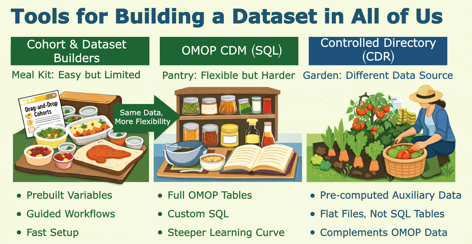
If you just scrolled past three SQL blocks and felt your eyes glaze over, good news: there’s a meal kit version. The AoU Cohort and Dataset Builders are point-and-click tools that work in two steps: define your participant criteria (the Cohort Builder), then build your data features (the Dataset Builder). Easy to use, but limited — like a meal kit, you’re working with what’s in the box. I didn’t find them flexible enough for my project, but they’re great for exploration. And since they run SQL under the hood, you can click “Analyze” → “See Code Preview” to peek at the BigQuery query they generated. It’s a handy starting point if you want to adapt it yourself.

Beyond OMOP-CDM: CDR Directory Files

Beyond observational data, note that some pre-computed data in the Researcher Workbench lives outside of OMOP-CDM data tables. If you have access to the Controlled CDR directory, you’ll find pre-computed genomic data (e.g., precomputed genetic ancestry, admixture estimates, relatedness, etc.) are made readily available in tab-delimited tables. These genetically-derived estimates can complement or replace the self-reported race and ethnicity values in the BigQuery tables.

Summary

That’s the full pipeline: find your concept IDs, query the right clinical table, label your coded values, and merge everything into a cohort. It takes more joins than UKB, but the logic is consistent once you’ve done it once. The next post moves from phenotype data into genotype data, where the complexity shifts from data models to file formats.